Fitness For Service – Metal Loss

Fitness For Service – Metal Loss

Fitness For Service General Metal Loss

One of the most common damage classes (modes) found in static mechanical plant is metal loss. It can be caused by a number of damage mechanisms such as;

-Atmospheric corrosion

-Erosion

-Sulphidation

-Corrosion Under Insulation (CUI)

-Microbiological Induced Corrosion (MIC)

-Under Deposit Corrosion(UDC)

-CO2 corrosion

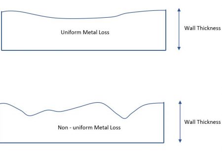
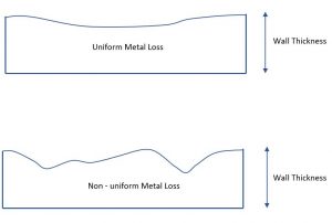
There are many more, and these can be found using  API RP 571, Damage Mechanisms Affecting Fixed Equipment in the Refining Industry. Metal loss can be further defined as ‘uniform metal loss’ and ‘non-uniform loss’. CAUTION! This is not the same as general metal loss and local metal loss! So, what’s the difference? Let’s take a look now.

When teaching Fitness For Service General Metal Loss, one of the most common questions we are asked is “how do you define general metal loss and local metal loss?”.  Well, there is no definition! API 579 Fitness For Service does not provide a quantitative assessment to determine whether the assessment should be treated under either Part 4 (General) or Part 5 (local) methods.  It relies on the assessor to determine the most applicable method. The general acceptance is that Part 4 can be completed first as a more conservative assessment, and if the component does not meet the level 1 criteria, then Part 5 can be considered.  (Other options are available such as Level 2/3 assessment, rerating, repair, replacement).

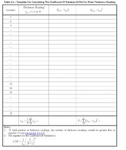
So, what about uniform versus non-uniform? How does this differ? Well, this is not about the extent of the loss, but rather the variance of recorded thickness readings. If you have ever studied statistics you will be familiar with the terms ‘Standard Deviation’. Determining whether the loss should be treated as uniform or not, all comes back to this. If the wall thickness readings are close together, then there is little variance and the loss is said to be uniform. If however, the wall thickness has a greater variance then the loss is said to be non-uniform.  We will use the Coefficient OF Variation (COV) of the thickness readings to conduct the assessment. The COV is the Standard Deviation divided by the average. The API 579 standard provides a table to assist you in computing the COV.

Let us look at how to conduct a Part 4 General Metal Loss assessment.

PART 4 LEVEL 1 – GML WORKED EXAMPLE

1. Pre-assessment Screening and Data Collection

Prior to undertaking any assessment, it is essential to identify the applicability and limitations of the procedure intended to be used. This can be found at the start of each Part of the method. The Part 4 GML Level 1 assessment applicability and limitations are summarised below.

Applicability

– For use when the metal loss exceeds or is predicted to exceed the corrosion allowance prior to the next inspection. In layman’s terms, anything that breaches the code required thickness or will exceed the code required thickness can be assessed.

– Only for the use of metal loss.

– Provides calculation methods for a de-rating of the MAWP.

– Component must not operate in the creep range.

– Only for Type A components subject to internal or external pressure (refer to API 579 for Type A components).

– Component is not in cyclic service (<150 cycles throughout its previous and future operating life, or satisfies the cyclic service screening procedure in Part 14).

– Smooth profile, i.e. no stress raisers.

– The area of loss must meet the minimum distance criteria from a major structural discontinuity.

A vessel insulation support or stiffening ring are examples of major structural discontinuities. 

2. Data Collection

To conduct a valid assessment, it is essential that the correct design, operating and inspection data is obtained. The following are the minimum requirements;

– Original equipment design data (list can be found in Part 2).

– Maintenance and Operational History (list found in Part 2).

– Point Thickness Readings (PTR) are used to characterise the metal loss when there are no significant variations in the thickness reading values.
1. A minimum of 15 thickness readings should be used unless the NDE method confirms metal loss is general.

2. If the Coefficient of Variation (COV) is greater than 10%, then thickness profiles readings should be considered.

3. Additional inspection may be required such as visual examination, radiography or other NDE methods.

– Thickness Profile Readings (CTP) are used when there is significant variation in thickness readings. In this case, readings are obtained from a grid and used to establish the CTP.

If CTP is used then the following procedure is performed to identify the required inspection points and the Critical Thickness Profiles.

1. To obtain the CTP a grid is drawn on the component and the readings taken at the intersecting points. The critical plane is the one that is under the most stress. For cylindrical shells under internal pressure loadings only, this will be the longitudinal plane. If bending or axial stresses govern, perhaps for poorly supported piping, then the circumferential plane may be the critical plane.

2. Mark each inspection plane on the component ensuring the length of the plane is sufficient to characterise the material loss.

3. Determine the uniform thickness away from the local metal loss location (trd), using UT or RT for example.

4. Take readings at the intervals along each plane, record the lowest remaining wall thickness (tmm).

5. Determine the CTP in the longitudinal and circumferential plane. This is simply taking the lowest reading from each point on the plane and projecting them into a common plane. The length of the profile is established by determining the endpoint locations where the remaining wall thickness is equal to, or greater than trd.

6. The length of this metal loss in the longitudinal direction is determined using the CTP and trd. In the example below, the red points indicate the lowest readings on each longitudinal plane, this is then projected onto a common plane and the length of loss measured. This length is denoted ’s’. (see figure  1)

7. The same process is followed for the circumferential plane and the length is denoted ‘c’. (see figure 1)

8. If multiple flaws are located in close proximity then the size of the flaw to be used in the assessment is obtained using the methodology in Fig. 4.11 of the Standard.

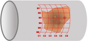
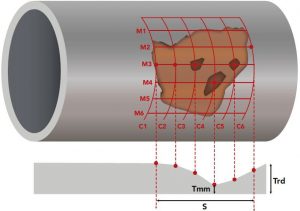
Fig. 1. Setting out the inspection grid.

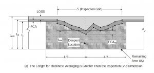
Fig. 2. Extract from API 579 displaying nomenclature.

The Standard provides a template to collate the required data and is titled ‘Table 4.2’. It is best practice to populate this table when collating the thickness readings prior to conducting the assessment. From a practical viewpoint, it is advisable to include the grid requirements in inspection work packs so that the required data is collected without further re-inspections.

Worked Example 1

During the inspection of a heat exchanger, internal corrosion was found on the cylindrical shell. The corrosion was caused by inadequate water dosing control which has now been improved. Determine if the heat exchanger is suitable for continued operation.

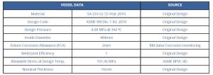
Inspection Data

Visual inspection confirms the corrosion loss can be characterised as general loss and point thickness readings will be used in the assessment. Please note that a minimum of 15 points are required to characterise the loss and perform a level 1 assessment; however, for the purpose of demonstration, this has been reduced to 5.

The table below provides the point thickness readings taken. It has been established that the uniform metal loss (LOSS) is 4mm (tnom- trd). See Figure 2

STEP 1 – Use the point thickness readings and determine the minimum measured thickness, tmm, the average thickness, tam, and the Coefficient of Variation, COV. The COV of the readings should be less than 10% otherwise thickness profiles (CTPs) shall be considered for use in the assessment. The COV is defined as the standard deviation divided by the average. The template for computing the COV is found in table 4.3.

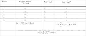
STEP 2 – The COV equals 0.0833 which is less than 0.1; therefore, we proceed to Step 3. If the COV was greater than 0.1 then the use of PTR is not permitted and the CTP would be used.

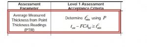
STEP 3 – To assess the acceptability of the component for continued operation, we must proceed to the relevant table. In this case Table 4.4 for cylindrical shells. Ensure to select the correct criteria, remember, we are using PTR in this case.

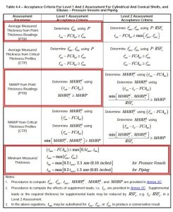
In this case, we used Point Thickness Readings, and so we must check the average thickness, minus any future corrosion allowance, meets the applicability criteria in table 4.4. Essentially, the average thickness minus future wall loss must not exceed the code required minimum thickness. It is essential to adjust any thickness and dimensions to account for the future metal loss.

Item does not pass Level 1 Part 4 assessment. Requires level 2 or the FCA factor reduced by arresting the loss. If the future metal loss can be arrested (through applying a coating for example) then none of the recorded thicknesses are below the minimum required thickness and the vessel is fit for service.

If the above criteria was met, then the additional check on the minimum measured thickness for structural protection must also be made, but we’ll cover that in the next article when we look at non-uniform loss.

If you are interested in training for fitness for service, why not check out our e-learning and classroom courses.